Authored by
Jonas Benner, Senior Quantitative Researcher
Stuart Eliot, Head of Portfolio Design and Management
This is the third in a series of educational notes about the role of store of value investments in a diversified portfolio.
In parts 1 and 2 of this series we explored the qualitative properties of Store of Value assets and assessed gold and Bitcoin against these properties. In this note we will take a more quantitative approach to better understand how including these assets in a diversified portfolio can impact its risk and return characteristics.
This is a long and fairly technical article, so we’ll start with a quick summary of the findings:
- In Section 1 we show that adding a modest amount of gold and Bitcoin to a standard diversified portfolio can both reduce the volatility and improve the returns of a model diversified portfolio.
- In Section 2 we show that it is reasonable to forecast that the same holds true on a forward-looking basis using traditional portfolio construction techniques, even when using somewhat modest return forecasts for gold and Bitcoin.
Section 1: Historical Analysis
Let’s start with the historical example (by modelling the historical performance of a hypothetical portfolio using actual historical data) and use it to examine a few important statistical concepts that will help us to understand how including gold and Bitcoin can change the behaviour of a portfolio. The Appendix to this note provides an explanation of each of the statistics and technical terms we use.
Our starting point is a hypothetical Simple Reference Portfolio (SRP) with 70% allocated to growth assets. It is constructed using the indices listed below, rebalanced to the target weights shown at the end of each month, and using month-end data from January 2001 to November 2025:
- 35% Australian equities (S&P/ASX Total Return 300 Index)
- 35% global equities, of which half is FX hedged (MSCI World ex Australia Net Total Return AUD Index)
- 12% Australian fixed interest (Bloomberg AusBond Composite 0+ Yr Index)
- 12% global fixed interest, fully FX hedged (Bloomberg Global-Aggregate Total Return Index Hedged AUD)
- 6% cash (Bloomberg AusBond Bank Bill Index)
Note: we use January 2001 as the starting point for this analysis as it is the earliest date for which AUD-denominated data for each of the component indices is available. See Box 1 in the Appendix for analysis of a USD-denominated portfolio going back to 1971. The below analyses do not include any fees, expenses or taxes.
Adding Store of Value assets (gold and Bitcoin) to the SRP
Now let’s examine the modelled performance of a portfolio that blends 5% gold with 95% of the SRP we discussed above.
| 2001 - 2025 | SRP | 95% SRP + 5% Gold |
| Returns | ||
| Cumulative return | 446% | 485% |
| Average annual total return | 7.2% | 7.4% |
| Average annual excess return | 3.6% | 3.8% |
| Risk | ||
| Average annual volatility | 8.4% | 7.8% |
| Number of drawdowns >5% | 7 | 6 |
| Worst drawdown | -31.3% | -27.7% |
| Average drawdown | -13.4% | -13.4% |
| Risk efficiency | ||
| Sharpe ratio | 0.42 | 0.49 |
Returns improve modestly, but what stands out is that many of the risk measures are meaningfully improved, resulting in an increase in the Sharpe ratio of the portfolio over the 2001-2025 period.
Let’s now repeat the same exercise with Bitcoin. For the calculations we will use 100% SRP from 2001 until March 2015 and then 5% Bitcoin blended with 95% SRP thereafter.
Bitcoin’s available price data starts in 2010; however, we will start our analysis from the end of March 2015 which we consider the date at which Bitcoin first became available to professional investors through the publicly available trading of the Grayscale Bitcoin Trust.
Between 2010 and 2015 the price of Bitcoin rose over 4000-fold. To include the pre-2015 data would of course flatter the analysis, but would also, in our view, invalidate it at the same time. The 2010-2015 period reflects Bitcoin’s transition from an experimental, thinly traded network into an investable asset, with extreme volatility, material market-structure frictions, and limited institutional access. Including it would mechanically dominate long-horizon portfolio outcomes and make the results less representative of the opportunity set available to professional investors today.
| 2001 - 2025 | SRP | 95% SRP + 5% Gold* | 95% SRP + 5% Bitcoin^ |
| Returns | |||
| Cumulative return | 446% | 485% | 693% |
| Average annual total return | 7.2% | 7.4% | 8.8% |
| Average annual excess return | 3.6% | 3.8% | 5.2% |
| Risk | |||
| Average annual volatility | 8.4% | 7.8% | 9.1% |
| Number of drawdowns >5% | 7 | 6 | 6 |
| Worst drawdown | -31.3% | -27.7% | -31.3% |
| Average drawdown | -13.4% | -13.4% | -15.6% |
| Risk efficiency | |||
| Sharpe ratio | 0.42 | 0.49 | 0.57 |
* 5% gold blended with 95% SRP for the entire 2001-2025 period
^ 100% SRP from 2001 until March 2015 and then 5% Bitcoin blended with 95% SRP thereafter.
Modelled returns improve materially, but most risk measures increase as well. Importantly, however, the Sharpe ratio increased from 0.42 to 0.57, meaning that the addition of 5% Bitcoin would have resulted in a large increase in risk efficiency.
Now let’s examine what would have happened if we divided the 5% modelled allocation equally between gold and Bitcoin, with the gold allocation at 5% until our March 2015 cut-off and then 2.5% allocated to each thereafter. An interesting thing happens!
| 2001 - 2025 | SRP | +5% Gold* | +5% Bitcoin^ | +2.5% Gold/2.5% Bitcoin~ |
| Returns | ||||
| Cumulative return | 446% | 485% | 693% | 595% |
| Average annual total return | 7.2% | 7.4% | 8.8% | 8.2% |
| Average annual excess return | 3.6% | 3.8% | 5.2% | 4.6% |
| Risk | ||||
| Average annual volatility | 8.4% | 7.8% | 9.1% | 8.3% |
| Number of drawdowns >5% | 7 | 6 | 6 | 6 |
| Worst drawdown | -31.3% | -27.7% | -31.3% | -27.7% |
| Average drawdown | -13.4% | -13.4% | -15.6% | -14.1% |
| Risk efficiency | ||||
| Sharpe ratio | 0.42 | 0.49 | 0.57 | 0.55 |
~ 95% SRP blended with 5% Gold from 2001 until March 2015 and then 95% SRP blended with 2.5% gold and 2.5% Bitcoin blended thereafter
While the Sharpe ratio of the modelled portfolio with 5% Bitcoin is the highest, it also comes with substantially higher volatility and more significant drawdowns. However, when we split the 5% modelled allocation to Store of Value assets equally between gold and Bitcoin, the result was to reduce risk slightly relative to the SRP on most measures, but to also meaningfully increase modelled returns, thereby retaining a large increase in the Sharpe ratio versus the original SRP.
If we put all four modelled portfolios together on a chart, we can see that each of the portfolios that include a Store of Value asset in their allocation outperform the SRP:
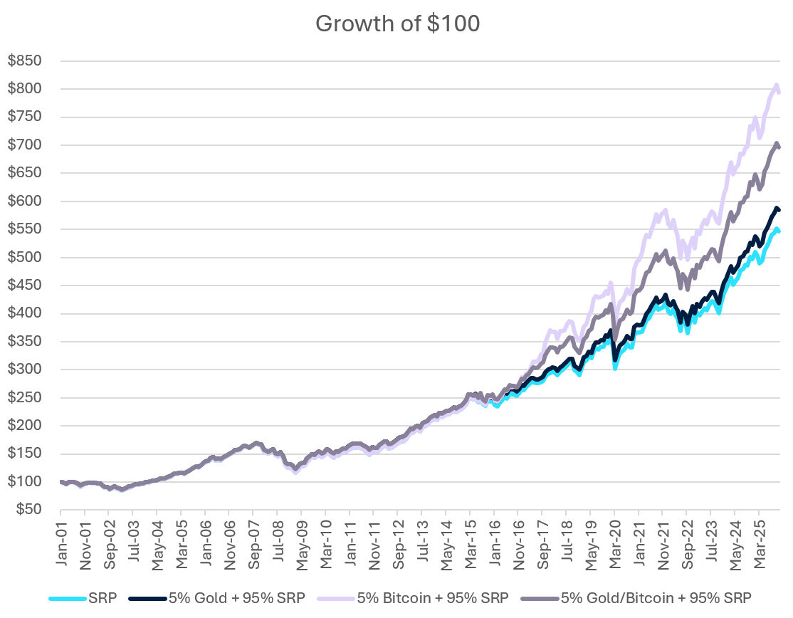
While this has been an interesting exploration of how simulating allocations to Store of Value assets would have improved portfolio outcomes in the past, it tells us little about building a portfolio today (and our lawyer insists that we remind everybody that “past performance is not a reliable indicator of future performance”). And so, we will now move on to the process of capital market forecasts and portfolio construction.
Section 2: Forward-Looking Analysis
In order to make a reasonable forecast of the expected return and volatility of a portfolio of assets we require 3 sets of data for all assets:
- Forecasts of volatilities,
- Forecasts of pair-wise correlations between assets,
- Forecasts of returns.
Volatility and correlation forecasts are readily available as they are typically calculated from historical data, and there are well-established methods for forecasting the expected returns of most assets. There are however (and somewhat surprisingly in the case of gold!) no widely agreed methods for forecasting the expected returns of gold and Bitcoin.
Price discovery tends to take place somewhere between that of a currency and a collectible (e.g., Fine art, vintage watches, BMX bikes, trading cards), as explored in detail in a fascinating recent blog post from Aswath Damodaran (Professor of Finance at Stern School of Business of New York University). Both gold and Bitcoin trade in high turnover, liquid markets with their price set against fiat currencies (typically the US Dollar) but there is no objective basis upon which one could argue that the price is either cheap or expensive – the price is the price. The price is simply where willing buyers and sellers agree to trade.
Our colleagues from the Macro Strategy and Economics team have provided us with their latest capital market forecasts, extending their volatility and correlation analysis to include gold and Bitcoin:
| Correlations | Cash | Aus Govt | Glob Govt | Aus EQ | Glob EQ (UH) | Glob EQ (H) | Gold | Bitcoin |
| Australian Cash | 1.00 | 0.28 | 0.39 | 0.02 | 0.06 | 0.00 | -0.02 | 0.16 |
| Australian Govt Bonds | 1.00 | 0.71 | 0.11 | 0.08 | 0.00 | 0.11 | 0.00 | |
| Global Govt Bonds (H) | 1.00 | 0.00 | 0.13 | 0.06 | 0.11 | 0.10 | ||
| Australian Equities | 1.00 | 0.45 | 0.64 | 0.19 | 0.08 | |||
| Global Developed Equities (Unhedged) | 1.00 | 0.79 | -0.05 | 0.16 | ||||
| Global Developed Equities (FX hedged) | 1.00 | 0.02 | 0.19 | |||||
| Gold | 1.00 | 0.01 | ||||||
| Bitcoin | 1.00 |
| Asset Class | Forecast Volatility % p.a. | Forecast Return % p.a. |
| Australian Cash | 0.5 | 3.75 |
| Australian Government Bonds | 4.0 | 4.25 |
| Global Govt Bonds (H) | 3.5 | 4.25 |
| Australian Equities | 16.5 | 7.25 |
| Global Developed Equities (Unhedged) | 14.5 | 7.25 |
| Global Developed Equities (FX hedged) | 14.5 | 7.25 |
| Gold | 13.5 | ? |
| Bitcoin | 50.0 | ? |
Which leaves the challenge of generating return forecasts for the last two rows.
Challenge accepted!
Let’s start with gold, borrowing again from the blog post of Professor Damodaran, the main reason to hold gold in a portfolio is as a hedge against crises and high rates of inflation, particularly if the bulk of a portfolio is invested in financial assets. (Real assets like land, property, and infrastructure should do relatively well in the presence of high inflation and therefore also make useful hedges.)
Starting with the assumption that the subset of investors who hold gold for these purposes hold a constant proportion of their portfolio in gold, this implies that the value of gold should rise and fall along with the overall nominal value of financial assets. However, given that this relationship is somewhat behavioural (i.e., the preference of investors to hold some proportion of their portfolio in gold for hedging purposes) we can expect that the proportion will vary with the perceived desirability of gold as a hedge or investment, which will be driven by factors such as gold’s recent price performance, fears of recession, inflation, and other crises.
Complementing this viewpoint, the World Gold Council published research in 2024 on Gold’s long-term expected return (GLTER) which explains changes in the value of gold as being positively related to nominal economic growth (i.e., inflation plus real GDP growth) and negatively related to market returns. Its conclusions are broadly consistent with the intuition that gold’s long-run performance is linked to inflation and macro regimes, though estimates vary across models and samples.
Gold as a safe haven
As a proxy for economic and market crises we have identified 9 occasions where the closing price of the S&P-500 Index declined by at least 15% from high to low since May 1982 (the first date for which we have data for US 10-Year Note futures). Included in this selection are the Global Financial Crisis, September 11, Covid-19, the Iraq invasion of Kuwait, the 2018 hawkish Fed and US-China trade war escalation, the 1987 crash, the LTCM hedge fund blow up, and “Liberation Day”.
For each of these ‘crisis’ periods we calculate between the dates of the S&P-500’s high and low:
- The change in the price of the S&P-500 Index
- The return of US 10-Year Note futures
- The return of gold.
Our choice of US 10-Year Note futures is because they are usually considered the go-to safe haven asset. They are highly liquid, perceived as likely to rise in a crisis, and are permitted investments in most diversified professional investment portfolios. However, we note that in inflationary or fiscal-stress regimes, bonds may be a less reliable hedge, which is one reason investors also consider complementary diversifiers.
| S&P High | S&P Low | S&P Price Return | 10-Year Note Return | Gold Return | Average of gold & bonds |
| 09-Oct-07 | 09-Mar-09 | -57% | 21% | 25% | 23% |
| 26-Mar-00 | 09-Oct-02 | -49% | 29% | 12% | 21% |
| 19-Feb-20 | 23-Mar-20 | -34% | 5% | -4% | 1% |
| 25-Aug-87 | 4-Dec-87 | -34% | -1% | 8% | 4% |
| 03-Jan-22 | 12-Oct-22 | -25% | -13% | -7% | -10% |
| 16-Jul-90 | 11-Oct-90 | -20% | -3% | 7% | 2% |
| 23-Sep-18 | 24-Dec-18 | -20% | 2% | 6% | 4% |
| 19-Jul-98 | 31-Aug-98 | -19% | 3% | -6% | -2% |
| 19-Feb-25 | 08-Apr-25 | -19% | 2% | 2% | 2% |
| Average | -30.7% | +5.1% | +4.7% | +4.9% | |
| R2 with S&P | 0.62 | 0.51 | 0.70 |
Gold outperformed 10-year note futures in 5 of the 9 crises captured in the table above, and one further occasion was a tie. Both hedging assets recorded positive returns in 6 of the 9 crises and the average return of 10-year note futures was marginally higher across the sample.
In comparison, the average return of bonds and gold was superior to either bonds or gold alone:
- The average return of both assets was positive in 7 of 9 crises, compared to 6 for either of bonds or gold = more reliable.
- The R2 between the returns of the S&P and the choice of hedging asset in the list of crises above was higher for the average of bonds and gold than for either asset individually = more predictable.
The conclusion that follows is not that one hedging asset is better than the other, but that a portfolio holding both gold and US 10-year notes would have been (and, we think, is reasonably likely to be) more effective in a crisis compared to a portfolio holding only one, or neither.
Towards a return forecast for gold
Bringing the above concepts together we can argue that:
- Gold has a useful role to play in a portfolio as a hedge against adverse events,
- There is a dollar value of gold that will be held at any given time for this purpose,
- This amount will be some function of the total value of all financial assets, the percentage of investors who choose to hold gold for its hedging qualities, and their desired portfolio allocation to gold for hedging purposes.
The first term in point 3 is an observable variable: the total value of investible assets. The second and third terms will be subjective, driven in part by collective concerns about events for which gold is considered to be a good hedge (e.g., inflation, currency debasement), and recent changes in the gold price.
This idea seems to have some validity based on existing data. For example if we compare the value of above-ground gold with the value of total financial assets (St Louis Fed data) the regression has an R2 of 0.90 indicating a strong relationship between the two over the long run.
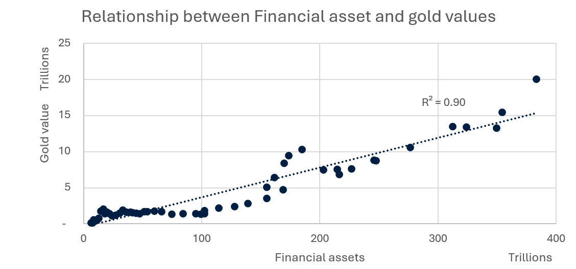
We observe a similar relationship between aggregate global money supply and the total value of gold. These relationships lend support to the idea of a central portfolio allocation to gold based on global financial asset values around which the total gold allocation moves depending upon the subjective factors described above.
From 1971 to the end of 2024 financial assets have increased at around 8% p.a. on average while OECD M3 Money supply and the value of above-ground gold have both increased at 10% p.a. on average.
Given that the value of gold appears to be a combination of the increase in financial asset values and a rational behavioural tendency, we think that it is reasonable to argue that the future will not differ meaningfully from the past and therefore the past should provide a good guide for the future in this regard. In a typical year, gold mining results in an increase in above-ground supply by less than 2%, contributing to the total value of gold in a way that doesn't benefit holders of gold, so we subtract this from the return forecast, and so…
We will therefore use the conservative forecast of 8% p.a. long term price returns for gold.
As a sense check, based on the other capital market forecasts above, 8% nominal annual return gives an excess return of 4.25% p.a. above cash. Dividing this by a forecast volatility of 13.5% gives a Sharpe ratio of ~0.3 which is a reasonable assessment of the rate at which gold converts risk into excess returns when compared to risk premia of other asset classes.
Forecasting Bitcoin’s returns
Now to Bitcoin’s return forecast, which requires more assumptions. Here we will rely on the assertion made in Part 2 that Bitcoin is an emerging store of value asset, with the implication of ‘emerging’ being that its share of overall store of value assets will therefore grow. For the reasons we covered in Part 2, we think that this is a reasonable assumption to make which then feeds into our forward looking statements below.
At the end of 2025, the combined value of gold and Bitcoin is ~$US33 trillion. Based on the 8% price return assumption for gold (as a proxy for store of value assets in total) plus around 1.75% annual mine supply this would increase to ~$US84 trillion by 2035. About $US13 trillion of this increase would arise from mining of gold and Bitcoin with the remainder of $US38 coming from price appreciation.
Assuming Bitcoin maintains its end-2025 5.3% share of store of value assets through to 2035 would imply annualised returns of 8.7% for Bitcoin and 8.0% for gold based on December 2025 prices. Under a constant-share scenario, Bitcoin’s implied price return is slightly higher because its future supply growth is lower than gold’s - meaning more of the required market-cap growth must occur through price rather than quantity.
By the time we get to 2035 Bitcoin will likely have either failed as a store of value asset or will have become more successful in capturing a greater share of the total store of value market. The table below reveals an interesting possibility, which is that if Bitcoin is able to become an equal partner with gold in the market for store of value assets, the price of gold could be little changed a decade from now. The implication is even if Bitcoin is successful as a store of value asset over the longer term, it may be prudent to hold both assets.
| Bitcoin SoV Capture | Bitcoin value ($T) | Gold value ($T) | Bitcoin price | Gold price | Bitcoin return p.a. | Gold return p.a |
| 0% | $ - | $83.32 | $ - | $9,586 | -100.0% | 8.6% |
| 5% | $4.19 | $79.62 | $201,285 | $9,107 | 8.7% | 8.0% |
| 10% | $8.38 | $75.43 | $402,570 | $8,627 | 16.5% | 7.5% |
| 15% | $12.57 | $71.24 | $603,855 | $8,148 | 21.3% | 6.8% |
| 20% | $16.76 | $67.05 | $805,140 | $7,669 | 24.8% | 6.2% |
| 25% | $20.95 | $62.86 | $1,006,424 | $7,189 | 27.6% | 5.5% |
| 30% | $25.14 | $58.67 | $1,207,709 | $6,710 | 30.0% | 4.8% |
| 35% | $29.34 | $54.48 | $1,408,994 | $6,231 | 32.0% | 4.0% |
| 40% | $33.53 | $50.29 | $1,610,279 | $5,752 | 33.8% | 3.2% |
| 45% | $37.72 | $46.10 | $1,811,564 | $5,272 | 35.4% | 2.3% |
| 50% | $41.91 | $41.91 | $2,012,849 | $4,793 | 36.8% | 1.3% |
Source: AMP
Taking a reasonably conservative approach in assuming that by 2035 Bitcoin doubles its share of the Store of Value market to 10.6% implies a return of 17.1% p.a. based on the method above, and so…
We will therefore use the forecast of 17% p.a. long term returns for Bitcoin1.
Again, applying the Sharpe ratio sense check, a 17% return with 50% volatility implies a Sharpe ratio below 0.3, which is consistent with other risk premia and similar to gold above.
Note that, for consistency this requires that we lower our forecast return for gold to 7.5% to reflect gold’s loss of store of value market share, which we have reflected in the analysis below.
Portfolio Construction
Now we are in possession of all the required inputs, we can generate an efficient frontier to help us understand the payoff between risk and return from adding gold and Bitcoin into our portfolio.
Our optimiser started with a base portfolio of the model SRP defined earlier and was allowed to substitute up to 5% each of gold and/or Bitcoin. For example, a portfolio with 4% gold and 2% Bitcoin would also contain 94% of the SRP.
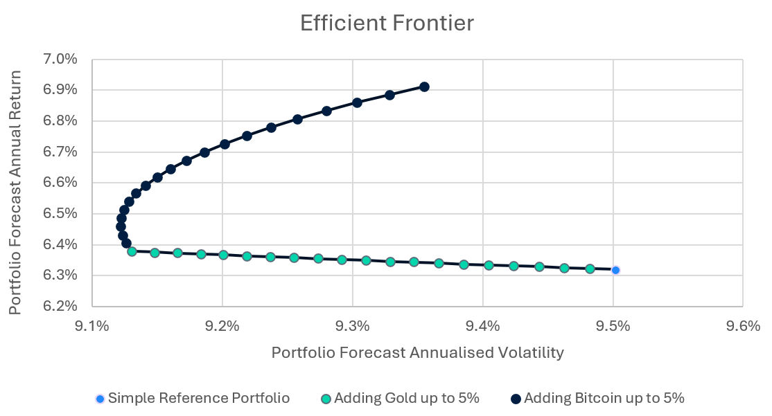
Two distinct phases are visible in the optimal allocations, with ‘optimal’ defined as the portfolio with the least volatility for a given level of expected return (equivalent to maximising the Sharpe ratio at a given level of expected return).
Phase 1 is the gently upward sloping straight line moving left from the SRP. As we progress further left along this part of the efficient frontier, the portfolio allocation to gold is increasing, expected returns are increasing and expected volatility is decreasing. At the far-left extent of this section of the efficient frontier the portfolio is allocated 5% to gold and 95% to the SRP.
Phase 2 is the curved section where the Bitcoin allocation is gradually increased from 0% to 5%, with gold remaining constant at 5%. At the very top of the efficient frontier the portfolio is allocated 5% to gold, 5% to Bitcoin, and 90% to the SRP.
Interestingly, adding Bitcoin does not immediately increase the forecast volatility of the portfolio: the minimum volatility portfolio subject to our constraints contains 5% gold and 0.75% Bitcoin. Furthermore, even with 0% gold in the portfolio, an allocation of up to 1.5% Bitcoin would result in lower forecast portfolio volatility than a 0% gold and 0% Bitcoin allocation.
But wait, isn’t this a bit biased?
A reasonable question at this point might be to ask whether we have rigged the numbers to make gold and Bitcoin look good in this framework.
To hopefully allay concerns of bias, we explored what returns one needs to believe are reasonable to justify any holding of gold and/or Bitcoin. It turns out that our optimiser will hold non-zero allocations to gold and Bitcoin, even when their forecast returns are lower than that of the SRP (which is 6.32%). Specifically, the optimal allocations to gold and Bitcoin rise above zero when forecast returns are equal to or greater than 4.2% and 5.8% p.a. respectively. Recall that these are less than the steady state returns of 8.0% and 8.7% calculated above using the assumption that the total market for Store of Value assets continues to increase at its historical rate over the coming decade.
The optimiser will reach the 5% maximum allocation when the forecast return for gold is 4.5% or more, and for Bitcoin when the forecast return is 9.4% or more. We believe these return expectations to be well within the realms of possibility.
Additionally, we would not be putting in the time and effort to write this series of notes if we did not strongly believe that store of value assets deserve a place in the portfolios of many investors.
You may also ask: isn’t this result just because your equity returns are too conservative?
We looked at that too. It turns out that with 12% as the return forecast for Australian and international equities, the optimal portfolio will hold the 5% maximum allocation to both gold and Bitcoin. Even if equities are forecast to return 15%, the optimal portfolio holds 5% gold and over 3% Bitcoin.
It turns out that gold’s diversifying characteristics are such that even if we forecast that equities would return an astounding 30% p.a. the optimal portfolio would still allocate a portion to gold.
In summary
The forward-looking analysis illustrates how incorporating gold and Bitcoin into a simulated diversified portfolio could deliver meaningful benefits, even under conservative return assumptions. We've demonstrated that both assets can be reasonably expected to enhance absolute and risk-adjusted returns while potentially also reducing portfolio volatility. This supports the case for including store of value assets within a diversified portfolio, acknowledging their distinct roles in hedging risks and capturing potential upside.
Looking Ahead: The Role of Alternative Diversifiers
In Part 4, the concluding part of this series, we will explore the potential role that alternative diversifiers can play alongside traditional diversifying assets within an investment portfolio. This discussion is particularly relevant for investors who are wary of the possibility that governments might pursue currency debasement to reduce their debt burdens. By examining these alternatives, we aim to provide insights into how portfolios can be further strengthened against such macroeconomic risks.
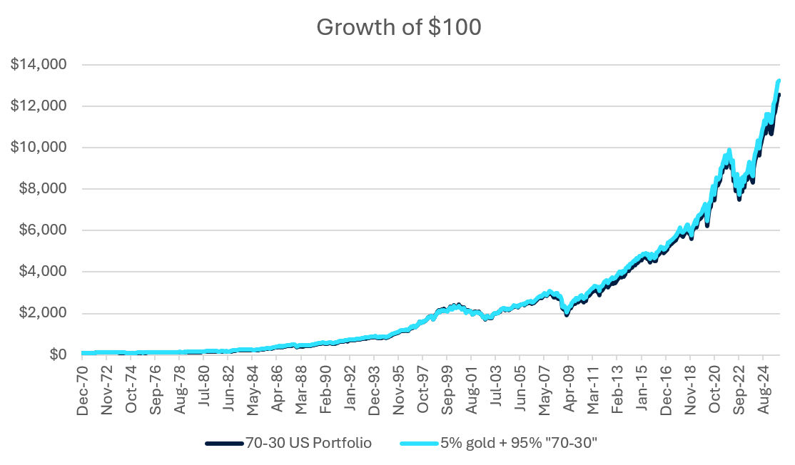
Box 1 - A Longer Perspective
To extend the analysis back to the start of 1971, we have created a simple diversified modelled portfolio which is 70% MSCI World US Total Returns and 30% constant maturity US government bonds. We compare this to a portfolio which is made up of 95% this simple portfolio and 5% gold. It could be argued that this simple portfolio is more difficult to beat (since it is more heavily weighted to US shares, which have performed exceptionally well in recent times) than the more globally diversified SRP discussed in the body of this article, and yet the substitution of 5% gold into the portfolio manages to do so anyway. The cumulative modelled return of the initial $100 portfolio containing gold is $711 higher after 55 years which is mainly due to compounding (and reduced variance drag, but that’s a topic for another article). The difference in average annual returns is surprisingly only 0.05%. The benefit is mainly driven by the reduced volatility of the portfolio containing gold (10.7% p.a. vs 11.2% without gold), making it a more risk efficient modelled portfolio.
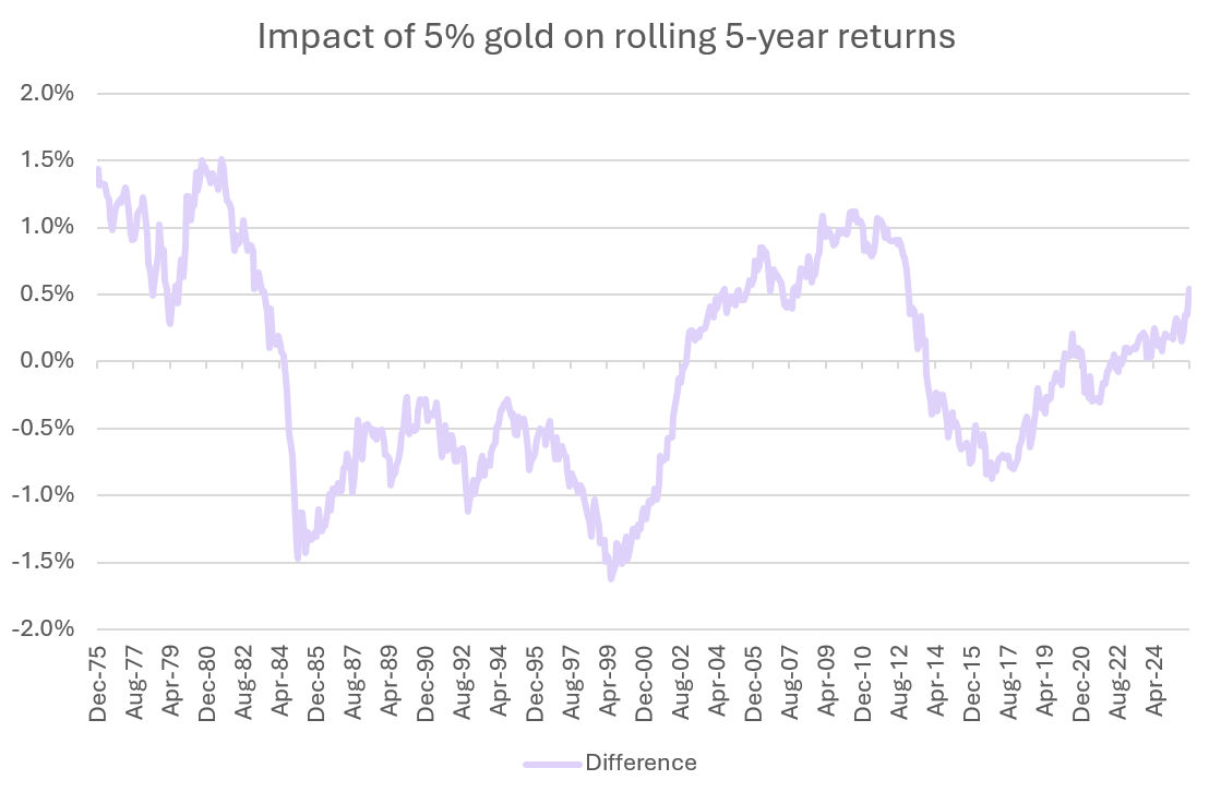
Looking at the rolling 5-year modelled returns, we can see that the inclusion of just 5% gold adds or detracts up to +/- 1.5% annualised over 5-year periods. We also observe that periods of out- or underperformance have tended to be episodic and that each episode has lasted for an extended period.
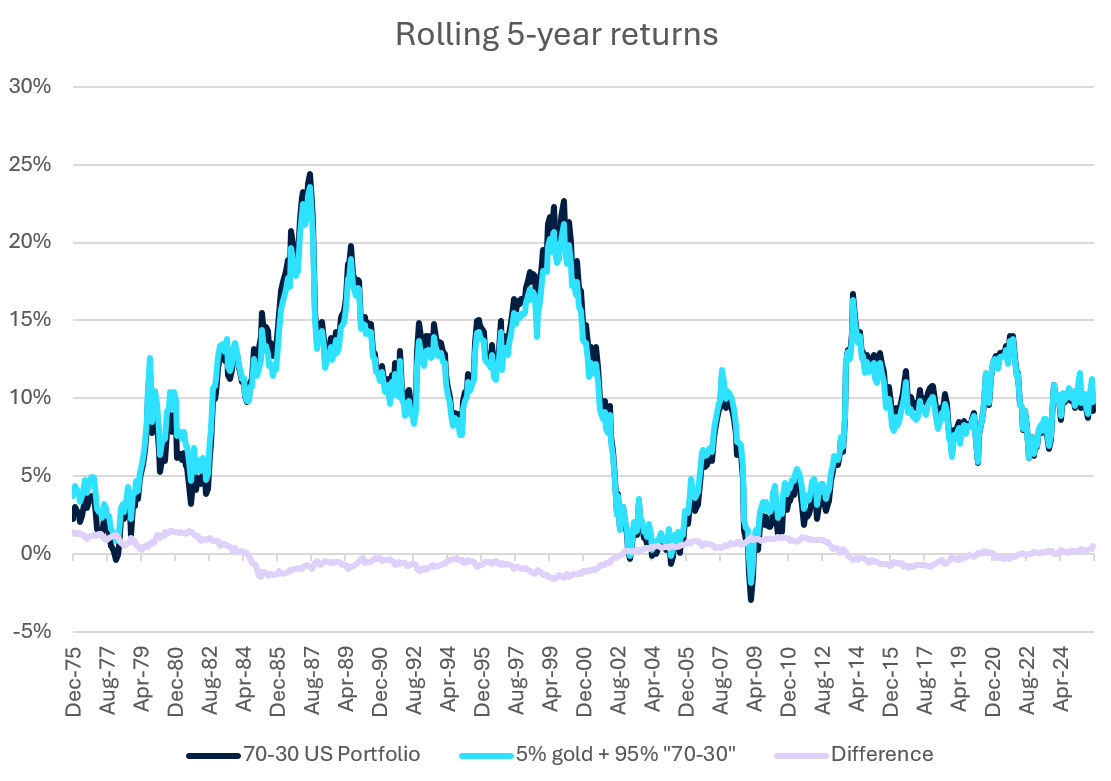
Gold added value to the simulated portfolio over 5-year holding periods up to 1984, then detracted until 2002. It then added value until 2013 and most recently began adding value to 5-year returns in 2022.
Measures of return and risk
We can calculate a range of statistics for a portfolio which fall into three distinct categories. Below we use the model SRP defined above as an example.
Return measures
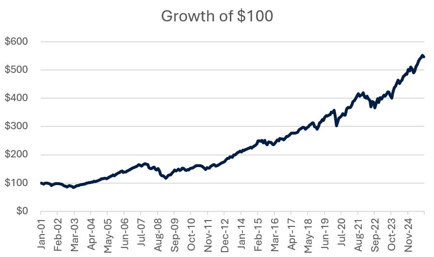
The first of these is cumulative return which is often expressed as the growth of an initial $100 investment. The cumulative return in the graph below is 446% ($546 vs $100). This doesn’t tell us a lot on its own but is useful in making a visual comparison of multiple investment strategies on the same chart.
The second is the average annual return, which is usually expressed as the simple average of monthly returns multiplied by 12. 7.2% p.a. for the SRP in the example above. (Although monthly is the convention we are using here, using other frequencies such as daily returns are valid too.)
The third is the average annual excess return, i.e., the additional return above this risk-free rate – cash in this case. This is calculated as the simple average of the difference between the portfolio’s return and the cash return each month, multiplied by 12. 3.6% in excess of cash for the SRP above.
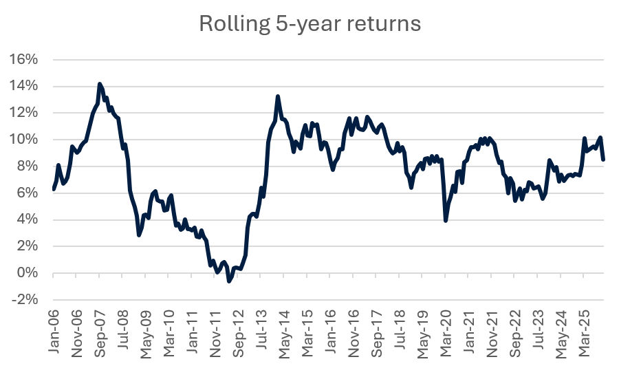
Finally, we have rolling total returns (or excess returns) which are simply the annualised cumulative return between a series of dates that are a fixed period apart. For example, the SRP’s rolling 5-year total returns look like this:
Risk measures
Portfolio risk is often expressed in terms of volatility, which is calculated as the Standard Deviation of monthly return multiplied by the square root of 12. (Volatility scales with the square root of time. Rather than providing a formal proof, it’s more intuitive to reflect that the variability of the price of an asset over a year is generally considerably less than 12 times its variability over a month.)
Our SRP has a volatility of 8.4% p.a., measured using either total or excess returns (the two are generally very similar).
The other main risk concept is that of a drawdown which is defined as the peak-to-trough decline in the value of a portfolio from a high-water mark. The drawdown ends when a new high-water mark is achieved. There are several clear examples of large drawdowns in the Growth of $100 chart above and numerous small drawdowns as well.
We can plot the drawdowns of our SRP as the distance the portfolio value is below a previous high-water mark as follows:
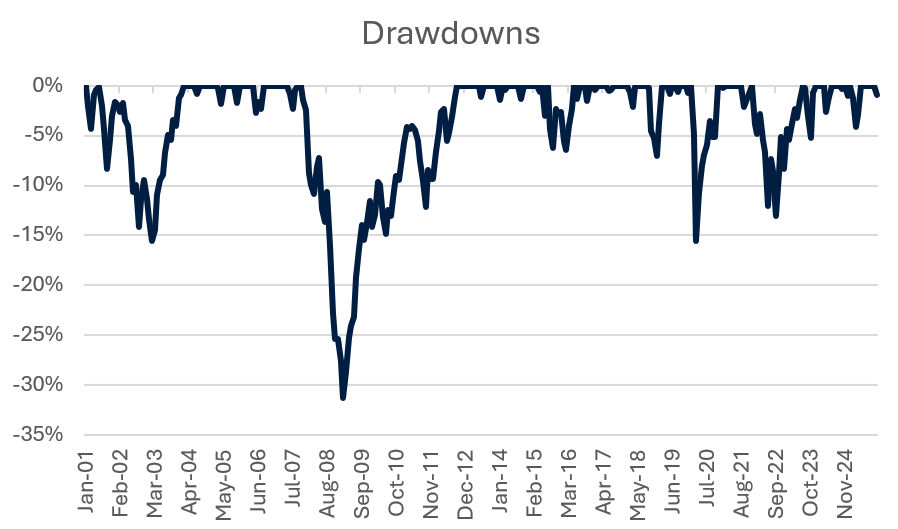
Any day that the portfolio is not making a new high is technically a drawdown, and so we need to choose a threshold to define what constitutes a drawdown to us. If we arbitrarily choose to define a significant drawdown as being a decline of 5% or more in the value of a portfolio, then we can extract several drawdown measures to compare different portfolios. In this case we have:
- 7 drawdowns > 5%
- Worst drawdown = -31.3%
- Average drawdown = -13.4%
Risk Efficiency
Our final portfolio statistic is the Sharpe ratio which is calculated as the portfolios excess return above the risk-free rate divided by the volatility of those excess returns.
We’ve already calculated both inputs for the Sharpe ratio above: 3.6% / 8.4% = 0.42
It’s helpful think of the Sharpe ratio as the rate at which risk is being converted into excess returns. One of the main goals when constructing diversified portfolios is to try to blend assets in a way that increases the Sharpe ratio. In other words, increasing expected returns relative to risk.
Other Metrics
R2 ,also called the “coefficient of determination”, is simply the square of the correlation coefficient. It measures how much two variables move together.
Currency of denomination
Both the gold and Bitcoin price are denominated in USD for this analysis.
You may also like

MyNorth Lifetime Conversations
19 July 2024 Our CEO, Alexis George recently caught up with Director and Principal Planner at CLS Investment Services, Mende Dulevski, to discuss MyNorth Lifetime and the impact that it's having on his business and clients. Read more
Why I use North - Mina Nguyen, Director of Essense Wealth
31 May 2024 In the latest instalment of our interview series with leading advisers, we caught up with Mina Nguyen of Essense Wealth. Read more
Amy's story
17 April 2024 Amy opens a MyNorth Lifetime Super account with a balance of $447,076. She has a $355,568 purchase amount, and potential age pension increase due to her 40% Centrelink discount. Read moreImportant information
The information on this page has been provided by NMMT Limited ABN 42 058 835 573, AFSL 234653 (NMMT). It contains general advice only, does not take account of your client’s personal objectives, financial situation or needs, and a client should consider whether this information is appropriate for them before making any decisions. It’s important your client consider their circumstances and read the relevant product disclosure statement (PDS), investor directed portfolio guide (IDPS Guide) and target market determination (TMD), available from northonline.com.au or by contacting the North Service Centre on 1800 667 841, before deciding what’s right for them.
MyNorth Investment and North Investment are operated by NMMT. MyNorth Investment Guarantee is issued by National Mutual Funds Management Limited ABN 32 006 787 720, AFSL 234652 (NMFM). MyNorth Super and Pension (including MyNorth Lifetime), MyNorth Super and Pension Guarantee and North Super and Pension are issued by N.M. Superannuation Proprietary Limited (ABN 31 008 428 322, AFSL 234654 (NM Super) as trustee of the Wealth Personal Superannuation and Pension Fund (the Fund) ABN 92 381 911 598. NMMT issues the interests in and is the responsible entity for MyNorth Managed Portfolios. All managed portfolios may not be available across all products on the North platform. All of the products above are referred to collectively as MyNorth Products. The information on this page is provided only for the use of advisers, it is not intended for clients. This page provides a brief overview of some of the benefits of investing in MyNorth Products. The adviser remains responsible for any advice/services they provide to clients including making their own inquiries and ensuring that the advice/services are appropriate and in accordance with all legal requirements.
You can read the Financial Services Guide online for more information, including the fees and benefits that companies related to NMMT, N.M. Superannuation Proprietary Limited ABN 31 008 428 322, AFSL 234654 (N.M. Super) and their representatives may receive in relation to products and services provided.
North and MyNorth are trademarks registered to NMMT.
All information on this website is subject to change without notice.
This article is for professional adviser use only and mustn’t be distributed to or made available to retail clients. It contains general advice only and doesn’t consider a person’s personal goals, financial situation or needs. A person should consider whether this information is appropriate for them before making any decisions. It’s important a person considers their circumstances and reads the relevant product disclosure statement and/or investor directed portfolio services guide, available from NMMT at northonline.com.au or by calling 1800 667 841, before deciding what’s right for them. You can read the NMMT Financial Services Guide online for more information, including the fees and benefits that AMP companies and their representatives may receive in relation to products and services provided. You can also ask us for a hard copy.
Past performance is not a reliable indicator of future performance.
This article includes forecasts, statements and estimates in relation to future matters, many of which are based on subjective judgements and/or proprietary internal modelling. No representation is made that such statements or estimates will prove correct. The reader should be aware that forward-looking statements are predictive in character and may be affected by inaccurate assumptions and/or by known or unknown risks and uncertainties. Results ultimately achieved may differ materially from forecast results. No independent third party has reviewed the reasonableness of any such forward-looking statements or the assumptions on which those forecasts are based.
The performance results in this article are hypothetical back test results for a model portfolio. They do not reflect the performance of actual investments. The back-tested results were achieved by means of the retroactive application of a model that was designed with the benefit of hindsight. This cannot reflect all of the complexities of actual investing and there are many material factors that would have affected actual results, including those relating to the markets in general, the impact of fees and expenses, liquidity activity and other factors, any or all of which may have adversely affected actual performance.
A number of the statements are based on information and research published by others. We have not confirmed, and do not warrant, the accuracy or completeness of that third-party information or research.